4  Hard X-Ray Telescope (HXT)

4.1  Preparations

Use YODAT to extract HXT data from the reformatted database. There are four key variables that are necessary for HXT data analyses described below: index, data, ssss, and infil. Here index, ssss and infil have similar contents as those in SXT data. The variable data contains compressed count rate data from HXT in the four energy bands. It has the form data = bytarr(4,64,4,m), where m is the number of major frames extracted from the reformatted database. The first ``4'' indicates the four energy bands of HXT, the next ``64'' indicates the 64 subcollimators (SC's), and the second ``4'' corresponds to the fact that HXT data appears four times in one major frame.

4.2  Time profiles

4.2.1  How to Plot Light Curves of HXT Data

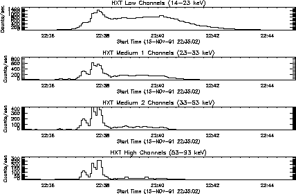
It is possible to get light curves of the four HXT channels on a single page by using the routine PLOTT_HDA. A sample plot is shown in Figure 4.5. If the HXT index or roadmap has already been read in using YODAT or another routine, then you can use the command:
 
IDL >  plott_hda, roadmap
You can also get HXT light curve plots by specifying a date and time. When you use this calling option with PLOTT_HDA it will use the HXT data stored in the Yohkoh observing log files, which is lower time and count resolution than accessing the data file directly. In the first example shown below, the data between 22:00 and 24:00 for 15-Nov-91 are plotted. In the second example, it will plot 30 minutes of data starting at 2-Dec-91 4:30.
 
IDL >  plott_hda, '15-nov-91 22:00', '15-nov-91 24:00'
IDL >  plott_hda,'2-dec-91 4:30',30

4.2.2  Displaying or printing time profiles

After extracting HXT data using YODAT, time profiles of HXT data in the four energy bands with the highest time resolution (e.g. 0.5 s for high-bit rate case) are displayed on the screen by typing:
 
IDL >  hxt_4chplot,index,data
with pre-storage of HXT data in DP taken into account (a four or eight second delay in the time tag for the data). Print-outs of HXT time profiles are available by adding an option /psout to the above command:
 
IDL >  hxt_4chplot,index,data,/psout
which produces a PostScript file ``idl.ps'' containing the time profiles on the current directory. The print-outs are easily obtained on Unix systems (which have the default printer set up properly) by typing
 
%  lpr idl.ps

4.2.3  Obtaining count rate data

HXT count rate data (in units of cts/s/SC) in the four energy bands are obtained by the following command:
 
IDL >  ave = ave_cts(index,data,time=time)
The count rate data are derived as an average of count rates from the 64 subcollimator outputs. The variable ave itself has no time tag in it. Instead, the variable time contains necessary information on time tag (pre-storage of HXT data taken into account). Time profiles of count rates in e.g. the M1 band are displayed by:
 
IDL >  utplot,time,ave(1,*,*),index(0)
This is just what is done in HXT_4CHPLOT.

4.3  Synthesizing Images from HXT Data

4.3.1   Determining the Flare Location on the Sun (HXT Address)

Before starting HXT image synthesis, we need to know the flare location on the Sun, in the HXT coordinates (whose origin is the HXT optical axis and unit is the HXT pitch (= 126^¢¢). East and north are positive). The most convenient way to do this is to run the following program:
 
IDL >  xy0 = get_hxt_pos('15-Nov-91 22:37')
Here '15-Nov-91 22:37' is the (approximate) date and time of the flare for which you want to make images. Values contained in xy0 (= fltarr(2)) are used in the next image synthesis procedure.

The routine GET_HXT_POS will perform the following checks in this order until it finds a match.

1. Read the $DIR_HXT_CAL/hxt_flare_pos.txt file to see if the time is in that list.
2. Use the GOES heliocentric location to determine the address
3. Use an SXT image index to define the address
4. Pass in heliocentric coordinates and convert them
5. Ask the user to specify the HXT address directly

See the Reference Guide for more details on GET_HXT_POS.

4.3.2  Quicklook of Synthesized Image (HXT_QLOOK)

HXT_QLOOK makes a series of HXT quick-look images (i.e. a quick-look movie). This program is much faster than the MEM code, but should be used only for quick-look movies. It is very useful for verifying positions before running a long MEM job. The HXT address of the flare location is needed even for this quick look synthesis, and it helps to use this routine to adjust the HXT address until a proper value is found.
 
IDL >  hxt_qlook, index, data, movie, hxi_index
IDL >  hxt_qlook, index, data, movie, hxi_index, patterns

See the Reference Guide for more details.

4.3.3  HXT_IMG (McTiernan) [*]

Jim McTiernan converted the FORTRAN program which was running on the mainframes to IDL. Currently the criteria used by HXT_IMG to stop the iterations is different from the FORTRAN program. HXT_IMG generally does not iterate as far. It takes a very long time to create a single image (between 1 and 30 minutes depending on the intensity) so we recommend running in batch mode when creating more than a couple of images.

1. The HDA data must be read into the variables data and index. A common way to do this is to use YODAT.
2. Now start running HXT_IMG by typing
    
   IDL >  .run hxt_img
   
3. Answer `No' to the first question (``Have the image synthesis parameters been loaded and modulation patterns been calculated?'')
4. Now comes the hard part. It is necessary to know the coordinates of the flare in HXT units (126 arcsec units). Please see the routine HXT_IMG_POS to see how to determine the HXT coordinates. For example, the 15-Nov-91 flare the coordinates were (-2.1, -4.8)
5. Answer `Yes' to the next two questions (use the default parameter files)
6. Select the channel you wish to have an image synthesized for
7. Answer `YES' for background subtracted
8. Locate a portion of the light curve where the signal is low (just background). Click with the left button on the plot at the start time, click with the right button at the end time, click the middle button to select the portion you have marked.
9. Locate a portion of the light curve where the signal is high where you want to have the HXT image synthesized. Click with the left button on the plot at the start time, click with the right button at the end time, click the middle button to select the portion you have marked.
10. The generation of that image will begin.
11. You will be asked if you want to save the results in an output file. That output HXI file can be read with YODAT or directly with RD_HXI.
12. When it is finished, the variables index_out and data_out will hold the results.

4.3.4  AUTO_HXI [*]

A driver for HXT_IMG was written which will automatically figure out how to integrate the HXT signal for each of the channels to accumulate 200 counts. The routine is very sensitive to the location of the flare and will not converge if the location is not correct. The flare is specified by selecting a time range and this means that the data files have to be in the directories that are returned by the DATA_PATHS routine (it figures out which files to use from the input times).

It figures out the location of the flare by (1) reading the GOES event log for the flare and converting the heliocentric coordinates, (2) converting the location of the SXT partial-frame images into HXT coordinates, or (3) to pass the location of the flare in the call to AUTO_HXI. The default is to do all channels, to use the GOES event location, to not subtract background, and to use a variable integration time to achieve 200 counts.

Some sample calls are:
 
IDL >  auto_hxi, sttim, entim
IDL >  auto_hxi, sttim, entim, chan=0
IDL >  auto_hxi, sttim, entim, chan=0, /sxt_pfi
IDL >  auto_hxi, sttim, entim, acc_cnts=[100,200,300,200]
IDL >  auto_hxi, sttim, entim, loc=[-2.1,-4.8]
IDL >  auto_hxi, sttim, entim, outdir='/yd8/scratch/morrison'
where sttim is the start date/time in any of the three standard formats (described in the Reference Guide), and entim is the end time. At this time, the routine performs no background subtraction before image synthesis.

4.4  Using HXT for Broad-Band Hard X-Ray Spectrophotometry

HXT has a large effective area. Accordingly, its four energy channels can be used for ordinary spectrophotometry via direct summation of the rates from the 64 independent detectors, independently of any application of these data to imaging. The data are well-calibrated and are normally free of any effects of pulse pile-up, owing to the small effective areas of the individual detectors. The four channels can be used to fit power-law or thermal spectra. The presence of spatial structure in the image affects the precision of the total-count photometry, but because there are 64 detectors, this effect is probably small.

4.4.1  Determining Temperatures

The program HXT_TEEM can be used to determine thermal fits to the data. It returns pairwise fits of the four channels, i.e., three independent values for temperature and emission measure. The instrument is sensitive to temperatures as low as 15 MK, but at the time of writing no systematic comparison of these temperatures with, say, those of the GOES photometers, had been carried out. The HXT_TEEM program has an interactive background determination feature that may make it easier to generate consistent temperature fits (Med1/Low and Med2/Med1) in the presence of the temporal variations of the background rates.

4.5  How to Fit HXT Spectra: HXTBOX_FSP (McTiernan) [*]

A general discussion of the McTiernan spectral fitting programs is given on page 6.3.1 in the description of fitting WBS spectra.

A routine which will do spatially resolved HXT spectra is also available, called HXTBOX_FSP. To use this, the input index and data structures must come from an HXI file, instead of index and data from HDA files used by HXT_FSP. The region for the spectral fit is chosen using the routine LCUR_IMAGE, before the time interval is chosen. Here are some sample calls.
 
IDL >  hxtbox_fsp, index, data, fit_pars
IDL >  hxtbox_fsp, index, data, fit_pars, boxq=boxq
IDL >  hxtbox_fsp, index, data, countfile = 'test.dat'
IDL >  hxtbox_fsp, index, data, fit_pars, same_bx=boxq
IDL >  hxtbox_fsp, index, data, fit_pars, boxq=boxq, /same_bx
where boxq is an array containing the subscripts of the chosen regions, (corresponding to the keyword marks in LCUR_IMAGE). If same_bx is set, the routine will use the array of subscripts contained in boxq (or if boxq is not set, than the array in same_bx is used). Note that the final two examples will accomplish the same thing. The output structure fit_pars is an array of (n_intervals × n_boxes).

4.6  Spectral analysis with HXT (Sakao)

As HXT has four energy bands between 14 keV and 93 keV, we can estimate incident hard X-ray spectra under certain assumptions about the spectral form (such as power law or thermal Bremsstrahlung emission) using count data pairs from different energy bands.

4.6.1   Background selection

Before starting spectral analysis, prepare background data using the following command:
 
IDL >  bkgd = mk_hxtdata(index,data,ssss,infil,channel=0)
In the above example, the time profile in the L band (channel=0) is displayed on the screen. Choose the background data interval in the same way as described in E.2 (4). Note that BGD data in all the four energy bands, which have the same start and end times specified from the L band time profile, are stored in the structure variable bkgd. The variable bkgd has the same structure as the one in E.2 (4); if you have already have the BGD data in your IDL memory, you need not run the above MK_HXTDATA.

4.6.2   Power Law Spectrum

If we assume an incident X-ray energy spectrum of a power law form: I(E) = A*(E/20 keV)^G (photons/s/cm²/keV), we can estimate hard X-ray flux at 20 keV (A) and photon index (G) by the following command:
 
IDL >  p = hxt_powerlaw(index,data,1,bkgd,time=time)
which provides us with time profiles of A (p(0,*)) and G (p(1,*)) with the highest temporal resolution (e.g. 0.5 s in high-bit rate). The number `1' in the above command specifies the lower band of a pair of two adjacent energy bands from which A and G are calculated; you can specify `0' (M1/L), `1' (M2/M1), or `2' (H/M2). The variable bkgd is the BGD data obtained in section 4.6.1. For example, a time profile of photon index is displayed as follows:
 
IDL >  utplot,time,p(0,*),index(0)
Values of p for each major frame are obtained by adding an option /sf to the arguments of HXT_POWERLAW:
 
IDL >  p = hxt_powerlaw(index,data,1,bkgd,/sf,time=time)
which is useful when the flare is not very intense and you need to accumulate HXT data to increase count statistics.

4.6.3  Thermal spectrum

If we assume that observed hard X-rays are emitted by single-temperature thermal Bremsstrahlung, then temperature (T (K)) and emission measure (EM ×10⁴⁸ cm^-3) of the thermal plasma is obtained by
 
IDL >  t = hxt_thermal(index,data,0,bkgd,time=time)
The variables t(0,*) and t(1,*) provide T and EM (in units of 10⁴⁸ cm^-3), respectively, with the highest temporal resolution. The arguments `0' and bkgd have the same meaning as in section 4.6.2. Option /sf is also available for this program.

4.7  Useful Routines for HXT

See the routines listed in the Appendix of this User's Guide on page A.3.