The following sections are intended as an extension of the ``Red Book'' paper which describes the fundamentals of the Soft X-ray Telescope (SXT). We strongly recommend that first time users read ``The Soft X-Ray Telescope for the Solar-A Mission'' which is in Solar Physics 136, pp 37-67.
Many sections in this chapter refer to the SXT Calibration Notes. A partial set of these notes can be found in the $DIR_SXT_DOC directory. Users should send a mail message to the account specified in the preface of this document if they want copies of the notes.
The SXT makes use of a front-illuminated, virtual-phase CCD to detect both X-ray and visible photon fluxes. While it is possible to operate CCDs in a photon counting mode, the SXT CCD is operated in a camera-integrating mode. This means that the shutter is opened for a short interval during which photon events are summed into the CCD's pixels. The amount of charge read out of the CCD by the camera represents the energy in the photon flux which has been integrated in each pixel, not the actual number of photons. If the incident beam is mono-energetic, then the amount of charge is directly proportional to the photon flux. However, since the Sun's X-ray flux is far from mono-energetic, we must model the response of the CCD for a given solar spectrum.
When a photon is absorbed in the CCD it produces electron-hole pairs in the silicon. The number of photons, N(g) that produced the charge or number of electrons, N(e-), which is read out of the CCD is given by
|
The CCD camera electronics contain analogue-to-digital converters. In this Guide the digital camera output is referred to as DN or Data Number. These values are read from the camera with 12-bit accuracy, but in the case of X-ray images, are compressed to 8-bit values using a pseudo-square root compression algorithm prior to being telemetered. Thus, when looking at raw SXT images, one should remember that the intensity values are typically compressed. The relation between the DN values and the integrated charge or number of electrons is given by
|
The effective area of the SXT to X-rays is described more fully in SXT Calibration Note 31 (J. R. Lemen, 11 Feb 93, Rev A) and also in SXT Calibration Notes 30 and 25.
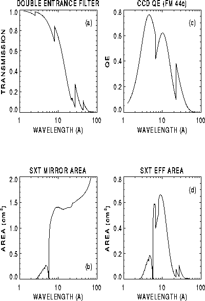
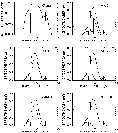
The on-axis effective area of the SXT depends on four different factors: the double entrance filter transmission, the mirror reflectivity, the analysis filter transmission, and the CCD quantum efficiency (QE). All these factors are functions of wavelength and off-axis angle (see section 4.3.4). Fig. 4.2 (a) shows the double entrance filter transmission, Fig. 4.2 (b) shows the mirror reflectivity (including the effects of obscuration by the support structures), and Fig. 4.2 (c) shows the CCD QE as a function of wavelength. Fig. 4.2 (d) shows the product of Figs 4.2 (a)-(c) and corresponds to the SXT effective area when both filter wheel positions are ``open'' and sometimes referred to in SXT documentation as ``noback'' (for no back filter). Fig. 4.3 contains six panels which show the SXT effective area through the open position and through each of the X-ray analysis filters. Calibration Note 31 gives details about how these curves were derived, but in short, measurements were made a selected wavelengths, to which model calculations were fit and used to predict the responses at any desired wavelength. NOTE: Be and Al12 are mistakenly reversed in Tsuneta et al. (1991) for Fig 4.4.
Although it is not normally necessary to access the effective are data file directly, it is
very easy to do so. In IDL you must type:
IDL > file = CONCAT_DIR('$DIR_SXT_SENSITIVE','sra930211_01.genx')
IDL > restgen,file=file, str=area
IDL > help,area,/str
	** Structure MS_125793397004, 5 tags, length=11600:
	   WAVE            FLOAT     Array(290)
	   ENTRANCE        FLOAT     Array(290)
	   CCD             FLOAT     Array(290)
	   MIRROR          FLOAT     Array(290)
	   FILTER          FLOAT     Array(6, 290)
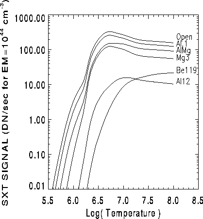
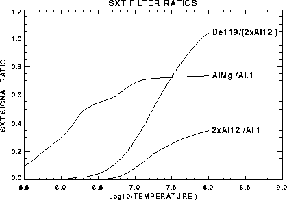
The response of the SXT to a thermal plasma has been computed using the thermal spectrum of Mewe et al. (1985, 1986), but with the abundances adjusted to coronal values (Meyer, 1985). The SXT thermal responses are shown in Fig. 4.4 for the various analysis filters. One can see from the curves that there are essentially two ``thick'' filters and three ``thin'' filters plus the open position. The open position has almost never been used during flight. This is because, prior to the entrance filter failure in November 1992, the aspect sensor door was left open almost continuously in order to take optical exposures. After the entrance filter failure in November 1992, the open position became unusable.
The SXT response functions are available through the IDL routine SXT_FLUX.
For example,
IDL > te = 5.5+findgen(51)*.05 ; Log10(te) vector between 5.5 and 8.0
IDL > plot_io,te,SXT_FLUX(te,1),yr=[.01,1000]
IDL > for i=2,6 do oplot,te,SXT_FLUX(te,i)
should reproduce Fig. 4.5. Note that the second argument is the normal
SXT filter-B number.
| 1 | Open/Open or Noback case |
| 2 | Al 1265 Å |
| 3 | Dagwood sandwich |
| 4 | Be 119 mm |
| 5 | AL 12 mm |
| 6 | Mg 3 mm |
The units of the plot are DN/sec for an emission measure, EM=1044 cm-3. SXT_FLUX has an optional switch: /photons; if specified, the routine will return the equivalent photons s-1 detected by the SXT. This will allow the user to determine the value of DN/photon as a function of filter and electron temperature. For example, try the following IDL commands to plot DN/photon for each filter as a function of electron temperature.
IDL > plot,te,SXT_FLUX(te,4)/SXT_FLUX(te,4,/photons) ; plot DN/photons vs te
IDL > for i=1,6 do oplot,te,SXT_FLUX(te,i)/SXT_FLUX(te,i,/photons)
The partial entrance filter failure in November 1992 caused a small
change to the SXT response function. SXT_FLUX has a date=
option which will return the new response function if the date is given
as date='13-nov-92 17:01' or later (the date can be given in any
standard Yohkoh format, such as a roadmap or index structure). In this
case, the fractional open area of the entrance filter (the size of the
hole) is taken to be 0.0833.
For information about how to obtain temperature estimates from the intensity ratios through the various filters, see the User's Guide.
The routine SXT_FLUX reads the thermal response function data from
a file. Although it is not normally necessary, the response function file can be read directly
using the following commands:
IDL > file=concat_dir('$DIR_SXT_SENSITIVE','sre930211_02.genx')
IDL > restgen, file=file, str=response
IDL > help,response,/str
	** Structure MS_125794338005, 5 tags, length=5280:
	   TEMP            FLOAT     Array(51)
	   ELECTS          FLOAT     Array(12, 51)
	   PHOTONS         FLOAT     Array(12, 51)
	   ELEM            STRING    Array(15)
	   ABUN            FLOAT     Array(15)
Note, that the response file may be updated from time to time. The name contains the date of the last update. In this data structure, the variable TEMP is Log10(Te), ELECTS are the number of CCD electrons (not DN) per sec for EM = 1044 cm-3, and PHOTONS is the corresponding number of photons. The first dimension of these two dimensional arrays is arranged so that columns 0 to 5 correspond to the filters in increasing thickness from 0=open to 5=Be119 and assuming the pre-launch entrance filter transmission. NOTE: This is not the normal SXT filter numbering scheme. Columns 6 to 11 correspond to the same filters but with no entrance filter. By combining the corresponding columns in the appropriate ratio, it is possible to quickly compute the SXT response for any size hole in the entrance filter.
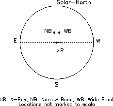
| x (East/West) | y (South/North) | ||
| NaBan boresight - X-ray boresight | -0.90 (±0.23) | +1.36 (±0.27) | final values (2008) |
| -0.36 (±0.18) | +1.47 (±0.28) | old values (1992) | |
| WdBan boresight - X-ray boresight | -0.25 (±0.23) | +1.08 (±0.25) | final values (2008) |
| +0.24 (±0.21) | +1.26 (±0.29) | old values (1992) |
where values are given in terms of SXT full-resolution (2.453 arcsec) pixels,
the negative values indicate East and South, respectively.
Fig. 4.6 shows the relative alignment
of the X-ray, narrow band and wide band boresights (as of 1992 analysis).
The most current values can be obtained with the routine GT_SXT_AXIS using the command:
IDL > print, gt_sxt_axis(1, /rel) ; NaBan -
> X-ray
IDL > print, gt_sxt_axis(2, /rel) ; WdBan -
> X-ray
A CCD pixel can contain about 3 ×10⁵ electrons before charge begins to spill into adjoining pixels. This effect is called ``pixel saturation''. The charge is not lost but appears in pixels surrounding (preferentially above) the saturated pixel. Exact saturation level varies from pixel to pixel but, in general, a signal level of DN=235 (compressed) in a full resolution image is considered to be saturated, i.e., the response of the CCD becomes non-linear. For half and quarter resolution, saturation occurs at DN=255 (compressed). These are the default levels used in SXT_SATPIX which is called by SXT_PREP. It is probable that DN=235 (compressed) is about 5% conservative as histograms of optical images indicate saturation setting in at DN=240 (compressed).
The 12 bit analog-to-digital-converter (ADC) of the CCD camera saturates at about 4.1 ×10⁵ electrons (4095 compressed to DN=255). Charge above this level is lost. Thus, the signal in saturated half or quarter resolution features is a lower limit.
The integrated X-ray intensity in a saturated full resolution image is not lost-only the spatial information is lost. The sum of all of the saturated pixels plus one pixel above (north) and one below (south) yields the integrated intensity of the area thus sampled. Only in very extreme cases does charge spill east or west into adjacent columns. NOTE that the signal in the pixel immediately above and below saturated pixels is questionable as it will usually contain spilled charge. We believe that the difference in saturation level between SXT X-ray and optical images is caused by the charge-spill effect which is not important for optical images - which have much lower contrast.
The routine SXT_SATPIX can be used to flag the location of saturated pixels.
Over time the SXT CCD collects some contaminant, whose origin is unknown. This is still happening, apparently at about the same rate, after more than 2 years in orbit! The problem is first apparent in optical images as noise in the form of short horizontal ``dashes'' randomly sprinkled over the image. Somewhat later, dark absorption ``freckles'' appear in the thin filter images at the same location as the ``dashes''.
The contamination is removed by heating the CCD to +20 C about every 3 months. Sometimes we have waited too long and these contamination artifacts are evident in the images. Although the effect of this contamination on observability of solar features is minimal, we have not yet quantitatively evaluated effects on things like measurement of temperature, emission measure, errors in intensity measurements, etc.
The periods of CCD bakeout are recorded in the appendix of the
Reference Guide and can be obtained with the program PR_DATES_WARM.
A sample call is:
IDL > pr_dates_warm
The CCD dark current increases about a factor of 2 for each 8 degree C increase in CCD temperature. The dark current at our normal operating temperature of -20 C is about 1 DN/sec for each full resolution pixel. Dark spikes or ``hot pixels'' have a corresponding rate of increase but, with a much higher dark current to begin with, can become quite dominant at CCD bakeout temperatures of +20 C. Although the analysis software tries to match dark frames of the appropriate temperature to the data being analyzed users should be alert for incorrect background subtraction during periods surrounding CCD bakeout. Dates of CCD bakeout can be obtained with the program PR_DATES_WARM and are listed in the appendix of the Reference Guide.
Areas of the CCD with high integrated X-ray dose, such as the east and west limbs, are observed to lose sensitivity for visible photons. The reason for this is still unknown. Thus, the aspect sensor images recorded before 14-Nov-92 when the entrance filter failed contain ``ghost images'' of the X-ray sun. The darkness of the ghosts fades with time to some degree.
For most uses of aspect images the ghosts have no effect. For quantitative studies with aspect images they may become important. Primitive flat-fielding routines are available. Hugh Hudson is the expert to consult.
The SXT operates through the South Atlantic Anomaly, for better continuity of coverage, even though the Yohkoh high energy sensors are switched off. SAA images are subject to lots of ``hot pixels'' and particle tracks from proton hits. These artifacts can be removed, to a fair degree, through use of the program DE_SPIKER.
In general, the background subtraction provided by SXT_PREP, DARK_SUB, and LEAK_SUB work amazingly well for such a complex problem. If background subtraction is a little off, substantial errors can accumulate in computing the intensity of large areas of faint emission. To better match exact exposure times the keyword /dc_interpolate should be used. For cases where even this is not satisfactory, the keyword /shift_floor will use the average of a 5×5 area in the lower left corner of the image as the background. This is usually only needed for the very shortest exposures.
Note that these routines leave the negative and zero values remaining from dark frame subtraction. These may need to be replaced with a positive value for, e.g., logarithmic display or ratio forming. By default SXT_TEEM will ignore negative intensity pixels when computing temperatures.
Dark subtraction will not remove cosmic or SAA artifacts which can be treated manually by replacing the offending pixel with the average of the surrounding pixels or through the use of DE_SPIKER.
After Nov-92, some background due to a visible light leak also needed to be removed. See section 4.3.5 for more details.
During fast transfer of a CCD image to reach the Region of Interest (ROI) of a PFI, charge builds up in the serial shift register of the CCD. This charge must be shifted out lest it bleed back onto the CCD and corrupt the image. A commandable guard band is provided to prevent this problem. However, on a few occasions charge bleed back is apparent in PFIs taken with the aspect sensor. The result is saturated columns appearing in the image, usually in the middle where 2 ROIs have been pasted together to create a 2 exposure PFI. A good (bad) example is
18-AUG-92 04:46:30 QT/H NaBan/Open Full Norm C 20 948.0 128x128There is no way to recover data corrupted by bleed back.
SXT has three on-chip summation modes available: full resolution (FR), half resolution (HR), and quarter resolution (QR). The pixel sizes are 2.45, 4.90, and 9.80 arcsec respectively. A factor to consider when working with images is the proper adjustments necessary when changing resolutions. The corner address saved in the index are the IDL CCD coordinates of the center of the binned pixel in the lower left corner.
Fig. B.17 on page B.17 shows some of the details of the CCD pixels, and how the pixels are summed on the CCD. Due to the camera design, the FR, HR and QR images are not perfectly aligned which each other. There is a shift of up to 3 full resolution pixels which needs to be accounted for when inter-comparing different resolution images.
There is also the age old question of whether to refer to the center of a pixel or to the corner of a pixel. We have decided to refer to the center of the pixel since it translates much better when working with fits between different resolutions.
See SXT Calibration Note 35 for a detailed discussion of the SXT CCD pixels and all of the various coordinate systems associated with the CCD: ground-based coordinate system using the camera system test set (CSTS), CCD readout pixel coordinate system, and others.
The DN value passed out of the camera when there is no light incident on the CCD and the dark current generation is zero will not be 0 DN. The minimum level is set electronically to be slightly higher, plus the spurious charge during readout causes another offset. The following are the approximate DN levels for no light incident on the cooled CCD.
This means that if you have one raw image (which has not had the dark current image removed) with an average signal of 15 DN and another with 20 DN, that is not a 25% difference, it is over 300% different. This offset must be watched carefully when working with low signal levels, even after the dark image has been removed.
The above values are appropriate for data acquired prior to 13-Nov-92. After the entrance filter failure, all values increased 1-2 DN due to a change in the spurious charge. NOTE: A separate effect is that the dark current has been increasing gradually during the mission, and will continue to do so, which is caused by X-ray damage.
DARK_SUB (which is what SXT_PREP calls), will remove a single dark frame which is closest in exposure level to the input image. When removing that single dark image, it takes off the digital offset, plus the dark current (exposure dependent) portion. An even better method is to use the /DC_INTERPOLATE option, which will interpolate two dark images to correct for the exposure dependent dark current, and will also remove the digital offset.
In order to extend the dynamic range of SXT for flare use, the forward filter wheel is equipped with a stainless steel mesh (``ND'' filter) with a transmission of 0.0805 �0.0008. While the mesh causes no noticeable degradation of the image it has been found to scatter X-rays (SXT Calibration Note 34) at about the 0.7% level. This is a minor effect for the brightest features in a flare but can provide the dominant signal in nearby faint features. No adequate means for correcting for this effect has yet been derived. Therefore, for greatest accuracy it is presently advisable not to mix images with and without the ND filter in determining the Te and EM of bright flare features and never to use ND filter images in the faint features. SXT_TEEM warns the user if the ND filter is included. E.g., the light curves, intensity, Te , and EM of faint areas of ND flare images may be totally in error. Because the scattering is diffuse and smooth, the images themselves are quite adequate as pictures of the flares for morphological studies.
The point spread function (PSF) of the SXT has a narrow core and wide scattering wings. Laboratory measurements of the core of the PSF have been analyzed thoroughly by Martens (SXT Calibration Note 34). The shape of the PSF is well characterized by an elliptical Moffat function with a FWHM of about 1.5 CCD pixels (3.7 arcsec) over the central area (diameter = 470 pixels or 2300 arcsec) of the CCD. Between a radius of 1 and 10 CCD pixels the slope of the PSF falls off roughly as a power law of index -4.
There is as yet no released software for deconvolution of SXT images, although McTiernan has done some work on this using the maximum entropy method and Roumeliotis has used a modified Lucy method.
The scattering wings of the SXT PSF begin to dominate the narrow core at about 20 arcsec from the center-at a level about 5 or 6 orders of magnitude down from the peak (see Fig. 4 in the Tsuneta, et al. (1991 `Red Book'). The scattering wings may be characterized from over-exposed flares observed in FFI mode such as 6-Sep-92 18:48. Hara (to be published) has derived the following expression which describes the shape of the PSF wing for a flare of 6.9×10⁶ K, through the thin filters
|
|
Scattering wing corrections have not yet been derived for the thicker filters and programs for use of the preliminary algorithms derived by Hara have not yet been released for general use because of concerns of their applicability away from sun center.
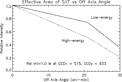
There are no fully approved routines to remove or correct for the SXT vignette function, however, there are a two preliminary routines. SXT_VIGNETTE will compute the vignette function as it is currently understood. The form and parameters of the shape may be changed as additional data and analysis become available. The routine SXT_OFF_AXIS will correct for the vignette function by calling SXT_VIGNETTE. Users are warned that these routines are preliminary and may not be the most appropriate technique to use, depending on the scientific application. However, they are certainly more accurate than no correction when intensities from different parts of the CCD must be compared.
The SXT entrance filter consists of a small amount of titanium and aluminum deposited on Lexan. In order to guard against the possibilities of pinholes, two such filters were flown back-to-back with the Lexan surfaces facing each other. These filters cover the X-ray entrance annulus and are arranged as six back-to-back pairs, or twelve individual filters in all. On 29-Oct-92 between 04:30 and 06:30 UT it was noticed that the optical images contained an halo of diffuse light. On 13-Nov-92 at 16:50 UT the visible light images became completely saturated. It is now thought that in October 1992 one of the outer entrance filters broke either completely or partially. The resulting halo was produced by the light that leaked through the inner filter that was behind the broken outer filter. Once the outer filter failed, the inner filter had its Lexan surface exposed to solar UV radiation and after three weeks of continuous exposure, the Lexan material deteriorated, causing the filter to at least partially fail. The resulting hole in the entrance filter allows visible light to be reflected by the X-ray mirror into the focal plane.
From an analysis of the data acquired after 14-Nov-92 it has been calculated that the fraction of the open area is 0.0833. The SXT_FLUX and SXT_TEEM routines take this into account when computing the response functions. The effect is negligible for the thick filters and makes only a small effect for the thin filters, increasing the response slightly at longer wavelengths. No adequate explanation for the partial entrance filter failure has been determined. This value and the date are available from the routine GET_YO_DATES(/entrance,/verbose). Analysis and description of these artifacts are given in SXT Calibration Notes 38 and 39.
When the 8% transmission X-ray ND mask is used, the stray light intensity increases a hundred fold. This is not as severe a problem as it sounds because exposures using the ND filter are generally quite short.
It has proven possible to acquire images with the SXT between 10 and 30 seconds before optical sunset-for which the atmosphere completely attenuates the X-ray sun with little effect on the visible illumination. These ``terminator'' images are routinely taken through all combinations of SXT filters for use in subtracting this stray light signal. This correction, along with dark frame subtraction, is provided by the program LEAK_SUB which will be updated from time to time as the terminator data base and correction algorithms improve. At present, LEAK_SUB is not perfect and over/under correction can be a problem you should be alert for. Because of complexity and partial randomness (especially for the thin Al filter), perfect straylight correction will never be possible.
The CCD camera employs a 12-bit ADC but data are transferred to the DP (telemetry) as 8-bit numbers. For purposes of gain calibration and helioseismology it is important to maintain the full 12-bit accuracy. This is accomplished by commanding compressed data and the low-order 8 bits for the same region, and then restoring the full 12 bits (see the routine RESTORE_LOW8 described in the Reference Guide).
The compression of ADC numbers uses the following algorithm. Taking DN, or Data Number, to be the CCD digital camera output, and X the 8-bit compressed value, and M the 12-bit decompressed value,
|
|
|
These expressions are used by the routines SXT_DECOMP and SXT_COMP for decompression and compression, respectively.
The SXT compression algorithm is not lossless, and so the decompressed values, M, contain a small error due to decompression: dM = |DN-M|. The algorithm has been selected so as to make the decompression error, dM, comparable to the statistical uncertainty. The decompression error is given by:
|
For X-ray images the error introduced by the SXT data compression is less than counting statistics so the compression from 12-bit (out of the CCD camera) to 8-bit numbers loses little information. For aspect images the errors in counting statistics are far less than the data compression errors. In order to obtain the best statistical precision, the aspect images were often taken in both low-8-bit and compressed data modes separately. These are combined to provide full 12-bit precision through the use of the program RESTORE_LOW8. This procedure works best if the two exposures are close together in time to minizize the effects of spacecraft pointing drift and jitter.
The Automatic Exposure Control of the SXT is described in the ``Red Book'' and briefly in the Reference Guide. One aspect of the AEC algorithm is that if the image is overexposed, and the AEC software has reduced the exposure to the lowest exposure level possible, then the logic could insert a ``thicker'' filter to avoid saturation. This option is enabled or disabled by the sequence table. There has been confusion on occasion when the filter has changed for a given sequence ``slot,'' even when there has been no table upload, or change in DP mode or DP rate. In most cases, the change in filter was due to AEC Filter Alternation.
The bottom line is that if exposure and ND filter adjustment do not suffice to maintain the desired exposure a thicker or thinner filter could be selected. Beware of this when analyzing flare data and an unexpected filter suddenly appears in the sequence!
The azimuthal orientation of the SXT CCD is mis-aligned slightly with
respect to the Yohkoh spacecraft. Thus, if the spacecraft is oriented
so that the solar north direction is parallel to the ``pitch'' axis, in
the SXT images solar north will not be exactly aligned with the y-axis
of the CCD, but rotated a small amount counter clockwise. A useful
routine for displaying a diagram of the roll angle relationships is
HELP_ROLL. The precise roll angle was not measured prior to launch.
The value has been determined from in-flight measurements and continues
to be refined. It is approximately 1 degree. The value which is used
currently in the on-line software can be checked by typing:
IDL > print,get_roll(/sxt) ; Print SXT roll-angle (degrees)
When analyzing SXT images, one should be aware that the Yohkoh
spacecraft roll orientation varies slightly. GET_ROLL by default
returns the roll angle of SXT with respect to solar north, incorporating
the CCD roll-angle and spacecraft roll angle. GET_ROLL tries to read
the ATT database files if they are available (see the reference guide
for more information). The ATT database already has the correction for
seasonal variation that exists between the spacecraft's on-board definition
and the true solar north value. If the ATT database is not available, the
routine will return values based on a sinusoidal fit to the seasonal variations,
but which does not take into account the true S/C roll.
Observing regions (OR) are composed of 64×64 PFI ``blocks.'' The simplest observing region is 64×64, but quite often larger observing regions are used. For example, when the observing region is 256×192, there are 4 ``blocks'' in the E/W direction and 3 in the N/S. Because of the way that the SXT telemetry buffers work, it is necessary to take three separate exposures for a 256×192 observing region. The assembly of these ``blocks'' into an observing region is performed properly for over 99% of the observing regions, however, there is a special case when a problem can occur.
When the telemetry mode is FFI dominant (the full frame images get the larger portion of the telemetry), it requires four major frames to telemeter a single 64×64 PFI ``block''. If any of the first portions of the ``block'' (which is 64×16) is missing, it will cause the image to be assembled incorrectly because of a lack of telemetry information. Be aware of occasional PFI portions which are not aligned properly.
SFD images are prepared from long and short exposure FFIs to extend the dynamic range of a given image to about 1 ×10⁶. The program MK_SFD is used for this purpose. These images are used to make the SXT ``movie'' and are especially valuable for surveying the data archive. Users should recognize that the SFD images are automatically prepared on a production line basis as part of the data reformatting process and should be alert for artifacts and features which are not of solar origin. Also, some areas of the images will have smoothed data inserted to replace saturation-bleed regions.
While, in general the SFD data are quantitatively correct, quantitative analysis should generally resort to the original SFR files which, for a variety of reasons, will often have images which are not made into SFD images. Users wishing to make their own composite images from 2 or 3 images of different exposure are referred to the program SXT_COMPOSITE.
If you have any question about SXT software and/or instrument, or if you need any advice in SXT data analyses, contact: