Welcome to the analysis of Yohkoh data. This document is intended to help you use the Yohkoh software and to understand the Yohkoh databases and some of the instrument calibration issues. The Yohkoh software has been written mostly in IDL, or Interactive Data Language, which is a licensed software program available from Research Systems, Inc. In order to run the Yohkoh analysis software, you must have IDL Version 3.0 or later installed on your computer or workstation. The Yohkoh Guide assumes that the reader has some familiarity with IDL already. For specific IDL questions, you are encouraged to consult the IDL User's and Reference Guides.
The Yohkoh software is known to work currently on several Unix-based platforms (e.g., HP, Sun, Mips, DEC, SGI). It is also available for VMS computers, however, we recommend that Unix be selected for analysis of Yohkoh data if possible. The installation and upgrade procedures described in the Reference Guide support only Unix systems.
Before beginning, it may be helpful to refer to Chapters 1 and 2 of
the Reference Guide (Volume 2) which briefly describe the Yohkoh instruments
and also provide an introduction to the Yohkoh data and software
organization. More details about the instruments can be found in the
Instrument Guide (Volume 3). You will want to make sure the Yohkoh software
is set up on your computer. Talk to your local manager about
this or follow the installation procedure described in the appendix of
the Reference Guide for Unix-based machines. The installation
can be accomplished easily by those possessing a moderate amount of
Unix experience. Next, check that you have a .yslogin file on
your home directory. Then type the following command:
% source ~/.yslogin
You must type this command at the beginning of each new login session or
see the Yohkoh Reference Guide about how to customize your .login
or .cshrc file.
Next, if you have Yohkoh data files on your disk, you should be able
to start looking at data after typing:
% idl
to start the IDL software system. YODAT (described in the next section)
is the most common way to read Yohkoh data files and display various
information or, in the case of SXT, to display images. If you have not
yet copied any Yohkoh data files to your computer's disk, you will
probably want begin with sections C.1 and C.2 which describe how to read
the Yohkoh data archive tapes.
The Yohkoh observing log contains a wealth of information which is readily accessible for searches and quick comparisons between instruments. In the following example the format of the plots may not be exactly what you need, but it is important to realize how simple the PLOTY program was to write since the observing log data files already exist. There is a lot of potential in the observing logs which is not being tapped as of yet, but the following sections touch on a few capabilities which currently exist.
XSEARCH_OBS provides graphical front end access to the Yohkoh Observing Log.
The user can select search criteria and define various options for output
1.
The calling sequence is:
IDL > xsearch_obs
The following features are anticipated.
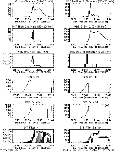
Fig. 2.1 is an example of the plot which can be produced. Note that the BCS counting rates drop to zero at around 22:37 because they become saturated. The format for the plots of this program might change in the future, but the capability to plot data from several instruments with the same time axes will remain.
TODO Needs text
There are a variety of routines which will produce listings of the images and pointing locations of the SXT partial frame images.
The routine PR_SXTOBS will read the observing log and list every FFI and PFI image
taken for the times requested. The format of the output is simply the output
of GET_INFO which is described in detail in the Reference Guide
(PR_SXTOBS simply reads the observing log and then calls GET_INFO). The command:
IDL > pr_sxtobs,'15-nov-91 22:00','15-nov-91 22:05',/long
will produce the output:
The routine SXTPNT_SUM will read the observing log and give a summary of the
unique PFI pointing for a given period. It groups the summary listing based on
each unique pointing location over time. The command:
It can be seen that the listing contains information on the number of images of a given filter
for each time span, the heliocentric coordinates, the NOAA active region number(s) if
applicable, the peak flux in HXT-LOW
and SXS2, the GOES flare event level, and a few other things. A ``*'' at the
end of the summary line says that the time of the peak of the GOES event
is contained within the time span shown.
The routine BCS_24HR_PLOT (discussed on page 3.1.3)
uses the data in the observing log by default, and
the routines PLOTT_HDA (discussed on page 4.2.1)
and PLOTT_WDA (discussed on page 6.1.1)
use the observing log if the calling sequence
specifies the starting and ending time. See the description and sample plots
of those routines described Sections 3.1.3, 4.2.1, and 6.1.1.
PR_EVN helps you find times for which Yohkoh data are available. An event is driven
by a change between QUIET and FLARE mode, or when there is a data gap of more
than 60 seconds. By typing:
A sample standard calling sequence for reading the observing log data files
for all instruments for a 12-hour period starting at 00:00 on 8-May-92 is:
XMOVIE_SFM, DISP_MONTH, GET_SFM
A laser disk movie exists at both ISAS and LPARL which contains SXT images
for the whole Yohkoh mission. These full frame images are all of the SFD
images which are available, which means 50-100 images a day for over two
years so far. It is possible to browse through the video recordings using a
remote control to look for events of a specific type or a specific time.
The routine VIDEO_MENU will allow a user to access the ``special laser
movie'' disk which has individual movies of particular events. See the
description in the Reference Guide for more details.
This procedure is run by typing (make sure that yodat is in lower case if
you are running on a Unix or Ultrix machine):
The ``MENU'' and ``MANY'' options search all data directories
which are returned by the function DATA_PATHS. At ISAS and LPARL this routine
automatically checks for new data directories that are on-line, in addition to
some ``hardwired'' directories which it always checks. It is possible for a
user to add directories to the list which DATA_PATHS returns by using the
routine NEW_DPATH. In the following example, the user adds the directory
``/yd3/morrison/agu_paper'' to the list of directories which will be
checked by YODAT.
If you selected data to be read, then the results are saved in the following variables:
For SXT options `SHOW_OBS3', `SHOW_OBS4', and `SSWHERE',
see the description in the Reference Guide.
The light curve options (all of the -400, -500, and -600 series)
will show a light curve of the selected channel. YODAT will prompt you
with the instructions at each step. It is possible to
select the range in time you wish to look at by:
An example of how one would use the -99 option is:
It is possible to use the -777 option to select SXT data by the sequence
table entry (all images taken with the same filter, resolution and field of view).
If you wish to abort from this option, click on the title
(the heading of the table). The most common technique is to just select
one sequence entry, but it is possible to select many entries. The
procedure is to select option -777, and then:
Another option is to use the -772 option to call SSWHERE which allows
the selection of SXT data based on filter, image resolution, DP mode
and rate, exposure duration, and several other options. See the
SSWHERE description in the Reference Guide for more details.
The BCS can provide detailed light curves and spectra.
After reading the BCS data with YODAT, you may wish to use the following commands:
Raw HXT data can provide light curves and spectra of the non-theraml emission in flares.
After reading the HXT data with YODAT, you may wish to use the following commands:
The SXT provides images of the thermal plasma in flare, active regions, and the quiet sun.
After reading the SXT data with YODAT, you may wish to use the following commands:
The WBS provides light curves and spectra from soft X-ray to gamma rays.
After reading the WBS data with YODAT, you may wish to use the following commands:
It is possible to perform spectral fitting on the HXT, WBS and SXT data by
using several routines written by Jim McTiernan. You can
fit three or more filters, and thermal and non-thermal spectra.
There are programs called SXTHXT_FSP and SXTHXTBOX_FSP,
which will fit combined spectra for the two instruments (SXT and HXT).
See the reference manual for details on how to run the program.
The WDEFROI function allows the user to select and cut-out an arbitrary
shaped region-of-interest (ROI) from a displayed image via point and click
with the mouse. With WDEFROI one can isolate a small intricately shaped
active region from a larger image for further analysis. This can be
particularly useful for reducing the computation time for calculating
temperatures and emission measures of large data cubes. WDEFROI is not SXT
specific, so it can be used on ground-based data or other derived data such
as temperatures and emission measure. One can obtain light curves of the
selected ROIs by passing normalized data and the times of data.
Example call to WDEFROI to obtain a sub-image via the keyword image:
The top row of buttons of this widget is used to pick the mode of ROI
selection and to change the color table (via XLOADCT). Below these buttons
is the online instruction box which displays useful general information and
specific information on how to make box, polygon, and contour selections
with the mouse. This is followed by some contour controls, namely a slider
widget which can be used to set the contour level at a specific value. Then
there is a row of control buttons: a select button to blacken-out all but
the selected area of the image; reset button to re-display the original image;
light curve to display a light curve of the selected area; exit to quit the
widget and to return to IDL command line. The final row has a display box
for the total number of pixels selected by box, polygon, and contour.
Example call to also plot light curves from normalized data:
Note: If the input data cube contains full frame images and the area of
interest is very small it may be best to call WDEFROI twice: 1st to isolate
the general area from the full context image and a second time with some zoom
factor to make contouring and extracting the smaller features easier.
PR_SXTOBS.PRO Run: 20-Dec-1993 21:06:29.00
SXT Observing Log Search from: 15-NOV-91  22:00:00 to 15-NOV-91  22:05:00

   0 15-NOV-91  22:03:40  QT/H  Open /Mg3   Half Norm C  17   338.0   64x 64  100%  S15W11   0%     41.3
   1 15-NOV-91  22:03:48  QT/H  Open /Al.1  Half Norm C  17   338.0   64x 64  100%  S15W11   0%     41.2
   2 15-NOV-91  22:03:56  QT/H  Open /AlMg  Half Norm C  19   668.0   64x 64  100%  S15W11   0%     41.0
   3 15-NOV-91  22:04:04  QT/H  Open /Be119 Half Norm C  27 10678.0   64x 64  100%  S15W11   0%     40.9
   4 15-NOV-91  22:04:18  QT/H  Open /Al12  Half Norm C  27 10678.0   64x 64  100%  S15W11   0%     40.7
   5 15-NOV-91  22:04:32  QT/H  Open /Mg3   Half Norm C  19   668.0   64x 64  100%  S15W11   0%     40.4
   6 15-NOV-91  22:04:36  QT/H  Open /Al.1  Half Norm C  23  2668.0  512x512  100%  Full D   2%     40.4
   7 15-NOV-91  22:04:44  QT/H  Open /Al.1  Half Norm C  17   338.0   64x 64  100%  S15W11   0%     40.2
   8 15-NOV-91  22:04:52  QT/H  Open /AlMg  Half Norm C  19   668.0   64x 64  100%  S15W11   0%     40.1
IDL > sxtpnt_sum, '5-oct-93 13:00', '6-oct-93 1:00'
will produce a file in your home directory with the name ``sxtpnt_sum.txt''
(unless you specify the output file name with the outfil keyword option).
The beginning of this file is:
OBS_SUMMARY  Ver 3.0
Program Run: 20-Dec-1993 21:12:40.00

      Date          Times          #Img  Mode    Table#    Filter A/B  Res  Exp  C DPE  msec    ImgSize  Loc   PntChange  NOAA

----------------------------------------------------------------------------------------------------------------------------------
  5-OCT-93  13:04:24 - 14:58:24    BCS: 441    SXTP: 146    SXTF:  19    W_H: 677     HXT-L:    1 SXS2:   16  S11E18
     5-OCT-93  13:04:24 - 14:56:50   39  QT/Hi    733/1  = Open /Al.1  Full Norm C  16   238.0  128x128 S11E18  (  0.2) [ 7592]
     5-OCT-93  13:04:42 - 14:57:52   37  QT/Hi    733/1  = Open /Al12  Full Norm C  24  3778.0  128x128 S11E18  (  0.2) [ 7592]
     5-OCT-93  13:05:14 - 14:58:24   36  QT/Hi    733/1  = Open /Al.1  Full Norm C  16   238.0  128x128 S11E18  (  0.2) [ 7592]
     5-OCT-93  13:05:54 - 14:56:18   34  QT/Hi    733/1  = Open /Al12  Full Norm C  24  3778.0  128x128 S11E19  (  0.2) [ 7592]
----------------------------------------------------------------------------------------------------------------------------------
  5-OCT-93  15:16:24 - 15:16:24    BCS:   0    SXTP:   1    SXTF:   0    W_H:   0     HXT-L:    0 SXS2:    0  S13E27
     5-OCT-93  15:16:24 - 15:16:24    1  QT/Hi    733/1  = Open /Al12  Full Norm C  24  3778.0  128x128 S13E27  (  0.0) [ 7592]
----------------------------------------------------------------------------------------------------------------------------------
  5-OCT-93  15:16:40 - 16:40:56    BCS: 190    SXTP: 133    SXTF:  15    W_H: 606     HXT-L:    1 SXS2:   16  S11E15      *
     5-OCT-93  15:16:40 - 16:40:56   33  QT/Hi    733/1  = Open /Al12  Full Norm C  24  3778.0  128x128 S13E17  (  0.7) [ 7592]
     5-OCT-93  15:16:56 - 16:39:20   35  QT/Hi    733/1  = Open /Al.1  Full Norm C  16   238.0  128x128 S13E17  (  0.7) [ 7592]
     5-OCT-93  15:17:28 - 16:39:52   34  QT/Hi    733/1  = Open /Al12  Full Norm C  26  7548.0  128x128 S13E17  (  0.7) [ 7592]
     5-OCT-93  15:18:00 - 16:40:24   31  QT/Hi    733/1  = Open /Al.1  Full Norm C  16   238.0  128x128 S11E15  (  0.7)
2.1.5 Light Curves from BCS, WBS and HXT
2.1.6 Creating a List of Yohkoh Events (PR_EVN)
IDL > pr_evn, '23-jun-92'
a list of the times that Yohkoh data are available and the number of datasets
available for each instrument is listed for 24 hours starting at 23-jun-92 00:00.
By typing:
IDL > pr_evn, '15-nov-91 20:00', '17-nov-91 15:00', /flare
all times that Yohkoh was in FLARE mode between those times are listed. By typing:
IDL > pr_evn, '1-jan-92', '9-jan-92', /flare, /counts, mindur=5, outfil='pr_evn.results'
the FLARE modes for 1992, and since the /COUNTS option was used, the maximum
counting rate for certain WBS, HXT, and BCS channels are printed instead of the
number of datasets available. It also prints the GOES classification when
it is available. The command shown above results in the following listing:
PR_EVN.PRO Run on  9-Dec-1993 12:07:26.00
Search Start Time:  1-JAN-92  00:00:00
Search End Time:    8-JAN-92  00:00:00
Minimum event duration:     5.00 minutes

NOTE: "*" means Yohkoh missed the beginning or end of the flare duration
      "+" means Yohkoh has a sub portion of data within the flare duration

     Start         End       Duration   DP           HXT    /         WBS                 /         BCS         / GOES
      (UT)        (UT)         (min)  Mode   Low  Med2 High /   SXS2   HXS   GRS1   RBMSD / Fe26 Fe25 Ca19  S15 /

 1-JAN-92  03:29:21-03:34:21   5.00  Flare     49    9    9 /    121    900    729      1 /  866 9676 5590 7586 / M2.8
 1-JAN-92  22:53:37-23:05:40  12.05  Flare      1    4    9 /    196   4624   7744      4 /  240  396  430 4083 /
 2-JAN-92  21:05:29-21:15:28   9.98  Flare     36    4    9 /     64    625    900      1 /  796 4210 9593 4340 / C9.3
 2-JAN-92  21:36:11-21:56:04  19.88  Flare     16    9   36 /    676  10000   7396      9 /  513 2210 3013 7290 / M1.9
 3-JAN-92  22:02:59-22:15:32  12.55  Flare      4    4   25 /    169   4489   7744     16 / 2083 3790 4573 9610 /
 4-JAN-92  08:48:43-08:58:40   9.95  Flare      4    9   16 /    256  24336   7396   4900 /   70  120  196 1276 /
 4-JAN-92  11:11:29-11:21:24   9.92  Flare     36    1    4 /     64    400    576      0 /  486 3150 2953 7210 /
 4-JAN-92  13:43:13-13:53:12   9.98  Flare     36    9    9 /     64   2809    576     25 /   80  490  883 3783 / C6.4
 5-JAN-92  13:15:33-13:25:14   9.68  Flare     25    4    9 /     64    576    784      0 /  626 4286 3930 6960 /
 5-JAN-92  15:14:55-15:24:20   9.42  Flare    576  961  196 /      4    441    841      0 /    0    0    0    0 /
 6-JAN-92  15:41:46-15:50:36   8.83  Flare    625  961  196 /      4    484    961      0 /    0    0    0    0 /
 6-JAN-92  19:55:06-20:09:39  14.55  Flare      4   16   36 /    400   7569   7225     16 / 3953  963  493 3903 /
 7-JAN-92  04:05:40-04:17:55  12.25  Flare     25    4    4 /     64    441    441      0 /  573 4196 4346 6420 / M1.5
 7-JAN-92  20:21:52-20:31:47   9.92  Flare     16    9   16 /     64   1764   2025     64 / 2116 1596 2000 4690 / C8.9
2.1.7 Direct Reading of the Observing Log
IDL > rd_obs, '8-may-92', '8-may-92 12:00', bcs, sxtf, sxtp, w_h, fid
An example for reading only SXT full frame entries is:
IDL > rd_obs, '1-jan-92', '1-jan-93', bcs, sxtf, /nobcs
Be aware that these datasets can get quite large so the time spans should probably
not exceed 10 days unless you are only accessing SXT full frame entries. See the
Reference Guide and the documentation header for RD_OBS for more details.
2.2 Summary SXT Full-frame image data
2.2.1 The Monthly SXT FFI files (SFM)
2.2.2 Browsing the Laser Movie (at ISAS, LPARL or MSU)
2.3 Accessing the Yohkoh Data
2.3.1
Interactive Access (YODAT)
YODAT will access any data from BCS, HXT, SXT, or WBS. It will also read
some FITS files which have been renamed to use the Yohkoh convention. This procedure:
IDL > .run yodat
The prompt that you will receive will look something like this:
% Compiled module: $MAIN$.
               *******  YODAT V9.2 (7-Jul-93)  *******

It is possible to have YODAT extract every "n"th dataset by setting
the variable QYODAT_NSAMP to 1.  You will be asked one extra question

It is possible to read the Ground Based Observation (GBO) FITS files
by using a command like: MENU g*
          gb_ files are from Big Bear, gk_ are from Kitt Peak
RFITS will be called with /SCALE option if QYODAT_SCALE is set to 1

Enter MENU if you want to use the filenames menu option
Enter SAME if you want to access the same fileID for a different instrument
Enter MANY if you want to use menu option and extract many files
Enter TIME if you want to enter the start/end time to extract
Enter QUIT to abort out of YODAT

Enter file name (or wild cards)
The first step is to select the data files to be read. The name of the file(s)
selected is saved in the variable infil. When one or more files are selected, the details of the datasets in
those files is read into the variable roadmap. There are several different
techniques for selecting files.
``/yd*/*/spr930623*'' or ``/yd6/flares/spr91*''.
IDL > new_dpath, '/yd3/morrison/agu_paper'
The second step in accessing any data set is to perform a quick review of the data available, and
select the data sets to be read. The options for selecting the data are
listed below.
Enter the number of data sets to extract
   * If you enter 0, all datasets will be extracted
   * If you enter -99, then it uses the datasets specified in variable "SS"
   * If you enter -888, then the file is not read
   * For SXT, enter a negative # (from -1 to -13) to access only that seq#
   * For SXT, enter -777 for sequence menu option
              Enter -776 to use "show_obs3" and select
              Enter -775 to use "plot_fov" and select
              Enter -774 to list the sequence summary
              Enter -773 to use "show_obs4" and select
              Enter -772 to use SSWHERE to select
   * For HXT, enter -666 to plot and select on SUM_L light curve
              Enter -665 to plot and select on SUM_M1 light curve
              Enter -664 to plot and select on SUM_M2 light curve
              Enter -663 to plot and select on SUM_H light curve
   * For WBS, enter -555 to plot and select on SXS1 light curve
              Enter -554 to plot and select on SXS2 light curve
              Enter -553 to plot and select on HXS light curve
   * For BCS, enter -444 to plot and select on S XV light curve
              Enter -443 to plot and select on Ca XIX light curve
              Enter -442 to plot and select on Fe XXV light curve
              Enter -441 to plot and select on FE XXVI light curve
   * For any, enter -333 to extract only flare mode data
infil the input file(s)
index the index structure for datasets extracted
data the data (array or structure) for datasets extracted
roadmap the complete roadmap for all datasets in infil
dset_arr the list of dataset numbers selected
info_array for SXT only, a text array describing each image
2.3.2 Advanced YODAT Options
2.3.3 Lowlevel Access Routine (READ_XDA)
2.3.4 Most Common BCS Display Routines
IDL > plott_bda, index ;light curve of all 4 chan
IDL > plott_bda, roadmap, psym=10 ;light curve of all 4 chan
IDL > wbda, index, data ;light curves and spectral plots
IDL > plots_bda, index, data ;spectral plot of all 4 chan
2.3.5 Most Common HXT Display Routines
IDL > plott_hda, index ;light curve of all 4 chan
IDL > plott_hda, roadmap, psym=10 ;light curve of all 4 chan
2.3.6 Most Common SXT Display Routines
IDL > stepper, data ;movie of data
IDL > stepper, data, xsiz=512 ;movie of data enlarged to 512x512
IDL > stepper, data, info=info_array ;movie of data with times...
IDL > xy_raster, index, data ;raster display of data
IDL > sxt_prep, index, data, index2, data2, /reg ;calibrate data
IDL > show_obs3, index ;time line of data
2.3.7 Most Common WBS Display Routines
IDL > plott_wda, index ;light curve of 7 sub-instruments
IDL > plott_wda, roadmap, psym=10 ;light curve of 7 sub-instruments
IDL > plots_wda, index, data ;simple spectral plots
2.4 How to Perform Spectral Fitting
2.5 Selection and Extraction of an Arbitrary Shaped Sub-Image (WDEFROI) [*]
IDL > sub_img = wdefroi(data, /image)
The program starts by bringing up the 1st image and running STEPPER
to allow the user to pick a working image frame from the variable data for
selecting ROIs (One can specify the working image frame by using the
sub=image_number keyword and avoid running STEPPER). Once the working frame
has been selected (say image 5), the user should exit STEPPER, and a widget
window will appear entitled WDEFROI.
IDL > sub_img = wdefroi(norm_data, /image, zoom=6, sub=5, /lc, time=index)
Where, norm_data is a data cube of small images say 64 by 64 pixels, zoom
specifies a zoom factor of 6, lc keyword requests light curve plot, and the
times for the light curve are passed via the time keyword.
Converted at the YDAC on Oct 4, 2004
(from LaTEX using TTH, version 1.92, with postprocessing)